Last Session — A Quick Recap
- ✓Variables & assignment
- ✓print() and f-strings
- ✓Built-in functions — len(), type(), round()
- ✓Four data types — str, int, float, bool
- ✓Arithmetic — +, -, *, /
- ✓.count() and a working GC calculator
…which is everything in the GC calculator you wrote:
name     = "BRCA1_exon3"
sequence = "ATGCGTACGTAGGCTA"

length   = len(sequence)
gc_count = sequence.count("G") + sequence.count("C")
gc_pct   = round(gc_count / length * 100, 1)

print(f"Gene:       {name}")
print(f"Length:     {length} bases")
print(f"GC content: {gc_pct}%")
From One Sequence to Many
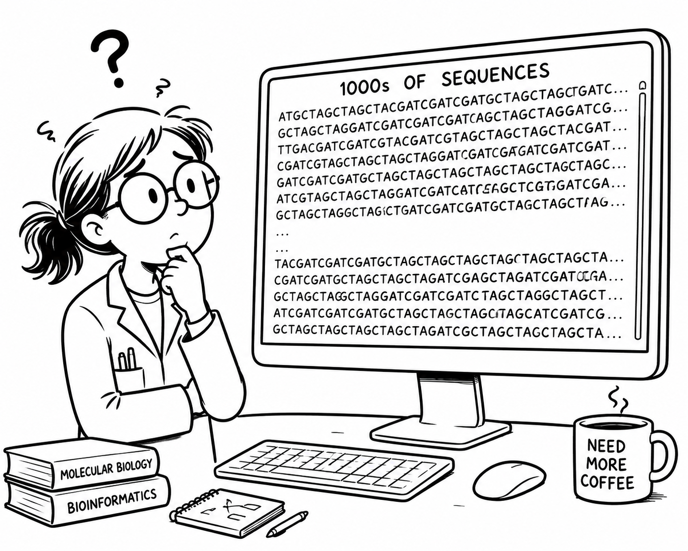
She can analyse one sequence. Now her supervisor hands her a whole folder of them. Making a separate variable — seq1, seq2, seq3… — for each one would be madness.
How do we move from handling one piece of data to handling many similar pieces at once? Python's answer is a container — and the simplest one is a list.
This Session — Data Containers
So far each variable held one value. Real data comes in collections — folders of sequences, tables of results. A container is a value that holds many other values. Today's three all share one idea: you reach inside with [ ].
An ordered collection — hold many sequences at once.
A string is a sequence of characters — reach in to pull out codons.
A lookup table — maps each codon to its amino acid.
Lists — one name, many values
Write the items between [ ], separated by commas. The order you write them in is the order they keep. len() tells you how many there are.
Run it, then add a gene of your own to the list and try running it again.
Reaching In — Index & Slice
genes[0] is the first item, genes[-1] the last. This trips up everyone at first — the first item is at position zero.
genes[1:3] gives items 1 and 2 — the end is not included.
Leave out the start (genes[:2]) or end (genes[2:]) to slice from the beginning or to the end of the list.
Run it — then try genes[2] and genes[1:-1]
Growing a List — append & join
The most common way a list grows: by adding items one-by-one to the end. This is exactly how we'll collect results inside a loop next session.
The same + you used to add numbers also joins lists end to end — just like it joins two strings together.
Run it, then try appending another gene before joining the lists.
Editing a List — replace & delete
Assign to a position — genes[1] = "KRAS" — and that item is swapped out. The list keeps its identity; only the contents change.
del genes[0] drops the first item; everything after it shuffles up. The list is now one shorter.
Run it — watch the positions shift after del. What happens if you del genes[-1] and then print the list?
Lists Hold Anything
A list doesn't care what it holds — strings, ints, floats, booleans — it can hold them all.
We could use one to hold a gene record: its name, length, GC fraction, and a Quality Control (QC) flag.
An item can itself be a list. Stack rows and you have a table; reach in twice — plate[1][0] — to get one cell. This is the shape of the data tables we'll meet later.
Run it, then try reaching into the table with plate[2][1] — which row and column does it print?
Lists of Numbers — sums & means
When a list holds numbers — replicate measurements, read counts, colony numbers — sum() totals them in one step. No need to add them by hand.
Pair sum() with len() and you have the average — sum(readings) / len(readings). The everyday workhorse of any analysis.
Run it — then add a sixth reading and watch the mean shift.
Try it Yourself — Clean the data, report the mean
You've just collected 20 readings from a growth assay in the lab. Clean up your data and then calculate the overall mean by following the steps below:
Scan with your phone — submit your mean value to today's poll.
A String Is a Sequence of Characters
A string holding a DNA sequence is just an ordered collection of bases. Reach in by position exactly as you did with lists:
dna[0] is the first base, dna[-1] the last, and len(dna) counts them.
Run it — then guess what dna[1] and dna[-2] will output. Try running them and see if you were right.
How Big Is a Character?
When text is saved or sent, each character is encoded as a pattern of bits. The worldwide standard is UTF-8, and it uses more bits for fancier characters.
With just four options, one base could be packed into 2 bits (A=00, T=01, G=10, C=11). But as an ordinary text character it takes 8 bits — four times bigger than it needs to be. Across a 3-billion-base genome, that waste adds up.
For squeezing whole genomes into memory, specialised tools pack 4 bases into each byte with bit operations. But for learning — and for almost every working biologist — a plain, readable ATGC string is exactly the right tool. Clarity beats cleverness.
Slicing Out Codons
seq[0:3] grabs the first three bases — one codon. Just like with lists, we use [start:end] to slice — remember that the end is not included, so 0:3 gives positions 0, 1, 2.
What if we want a slice in reverse order? We can set the step value. Using [::-1] moves backwards through the slice 1 step at a time — perfect for getting the reverse-complement strand.
Run it — then find out what happens if you step through every 3rd base with seq[::3]. Can you figure out how to slice the 3rd codon?
Building Strings — and why they don't change
The same operators you used on numbers and lists also build strings — primer + seq joins them, and "N" * 5 repeats the string.
Unlike a list, you can't edit a string in place — seq[0] = "T" is a TypeError. To “change” a string you build a new one with slicing and +.
Run it — then uncomment the last line to see the TypeError when you try to edit one character of the string in place.
String Methods — clean & search
Strings carry their own tools, called with a dot: seq.upper(). You met .count() last week — here are the ones you'll use the most.
Methods can be chained together — the output of one becomes the input of the next. seq.upper().find("GAATTC") makes the string uppercase, then searches for the EcoRI motif.
Run it — then try .find("TTT") to look for a motif that isn't there. How many "AT"s are in the sequence?
Transcription with .replace()
dna.replace("T", "U") returns a new string with every T turned into U — DNA transcription in one line.
Chaining .replace() to make a complement breaks: turn every A into T, then every T into A, and the A's you just made flip straight back. To complement each base independently we need a loop — that's Session 3.
Run it — if the final line made the complement, it would print TACGCA, but it doesn't. We need loops for this — next week!
Try it Yourself — Profile a sequence
One messy sequence in, a tidy summary out — using everything from this block. Clean it first, then answer each question in turn.
Scan with your phone — submit your answer to today's poll.
Dictionaries — a lookup table
A list finds things by position (0, 1, 2). A dictionary finds each value it holds via a paired key — here, a codon. Write the pairs in { } as key: value.
The genetic code is a lookup table: each three-base codon maps to one amino acid. That's a dictionary, exactly.
Run it — then add a fourth codon of your own (you can make it up or find one online!).
Dictionaries Are Everywhere
Any time data comes with labels, a dictionary fits. It's the most common way to store structured data in Python — config files, web data (JSON) and results tables are all dictionaries underneath. And the value can be anything:
{
  "red_fox": 12,
  "rabbit": 340,
  "buzzard": 5,
}
Species → count. The value is a number.
{
  "neuron_1": [12, 45, 78],
  "neuron_2": [9, 33],
}
Neuron → spike times. The value is a list.
{
  "p_01": {"age": 34, "bp": 128},
  "p_02": {"age": 51, "bp": 142},
}
Patient → record. The value is another dict.
Numbers, strings, lists, even other dictionaries — that flexibility is why dictionaries turn up in every field.
What's in my dictionary? Keys, values & items
What if we want to look up just the keys or the values in our codon table? We can use the .keys() and .values() methods to do that.
Sometimes we want to see both the key and the value together. The .items() method returns all of the key–value pairs in the dictionary. We'll be using it in the next lecture.
Remember, each item in a dictionary maps a key to a value.
Looking Up a Value by its Key
The same [ ] you used to reach into lists and strings — but instead of a position you give the key, and Python hands back its value. One step, instant answer.
Run it — then look up "GGT".
When the Key Isn't There — .get()
codon_table["TTT"] stops your program if TTT was never added. Real data is full of surprises — you need a safer way to ask.
If the key exists you get its value; if not, you get the fallback you chose — "?" here. Perfect for an unknown or malformed codon.
Run it — then uncomment the ["TTT"] line to meet the KeyError.
Building & Checking
table["TAA"] = "Stop" adds a new entry. If you use a key that already exists, it overwrites the old value — no error, no duplicate.
"ATG" in codon_table answers True/False — your loop-free way to search for a key. len() counts the entries.
Run it — watch GGT get updated, not duplicated. Then try adding a new codon!
Try it Yourself — Translate by lookup
This task fuses both halves of today — slice a codon out of the sequence, then look it up in the table. One codon is deliberately missing.
Scan with your phone — submit your answer to today's poll.
Recap — Lists, Strings & Maps
You started with one sequence and ended up translating it by hand — slicing out codons and looking each one up in a table. Three new containers got you there.
- ✓Hold many values in order
- ✓Index & slice — seq[0], seq[0:3]
- ✓.append() to grow, [i] = … to edit
- ✓sum() / len() over a list of numbers
- ✓A string is a sequence too
- ✓Slice out codons — seq[3:6]
- ✓Immutable — methods return a new string
- ✓.upper() .find() .replace() (transcription)
- ✓A lookup table — key → value
- ✓The codon table: "ATG" → "Met"
- ✓Look up with [key]; .get(key, "?") is safe
- ✓Add / update by key; test with in
What's Next — Programs That Run Themselves
Today you translated three codons by hand. But a real gene has hundreds — you can't write a line for each. Next time we hand the repetition to the computer, so it can run through a whole sequence on its own.
- ▸Loops — repeat the lookup for every codon, not just three
- ▸Conditionals — if / else to make decisions ("is this a stop codon?")
- ▸Combine them — walk a whole gene and stop when you hit a Stop
- ▸The program decides what to do — it runs itself
You now have every piece a translator needs — a sequence, a way to slice it, and a table to look codons up in. Control flow is what turns those pieces into one autonomous program.
- →Re-open today’s Colab notebook and re-do the codon translator
- →Try it on a longer sequence — notice how tedious three-by-three gets
- →Half an hour of practice beats re-watching the lecture
See you next week!