Python for Biologists

Last week you asked the table

You loaded a CSV, filtered it, grouped it, and got an answer out — all of it as numbers in a terminal.

You can already do this

read_csv, .groupby(), .mean() — enough to answer a real question.

But you had to read it

Eighteen rows of numbers. You found the answer by scanning down a column with your finger.

Today the computer does the looking.

Some patterns are invisible in a table and obvious in a picture — the difference between finding a result and walking past it.

Today: plotting figures

The data

DepMap

1,165 cancer cell lines, every gene switched off one at a time.

The question

Who needs SOX10?

Most cancer cells don't care when it is gone. Some die. Which ones?

The technique

Figures with matplotlib

One way of plotting, learned slowly and done properly.

DepMap: which genes does a cancer need?

1 · Grow the cells

1,165 cancer cell lines from 30 tissues: skin, lung, bowel, blood…

2 · Break one gene per cell

CRISPR: every cell gets a guide that knocks out one gene. Together the guides cover every gene.

3 · Let them grow

About three weeks. Cells that lost a gene they need die or grow slowly.

4 · Count the survivors

Sequence the guides. Guides for essential genes have gone missing.

The number: gene effect

−2−10+

0 the cells did not care
−1 as bad as losing a typical essential gene
below −1 even worse
positive better off without it

Lower = more needed. depmap.org

⏳Python editor will load when you reach this slide.

Part 1

How a figure shows data

Before any code: what kind of data you have decides which plot to draw, and how to show a difference: by position, colour, shape or size.

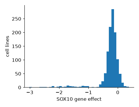
A figure is worth a thousand numbers

The gene SOX10 across all 1,165 cell lines, twice: as four numbers, and as a picture.

⏳Python editor will load when you reach this slide.

The mean says −0.27: a gene that barely matters. The picture says 93 cell lines genuinely need it — averaged away by a single number. Who are they? That is today's case.

Two kinds of data: categorical and continuous

Every column you will ever plot is one of two kinds. Work out which before you choose a plot: the plot follows from it.

Categorical

labels you can count

Examples: cancer lineage (Skin, Lung, Bowel…), cell line name, genotype (mutant / wild type), treatment

The test: Is “halfway between” meaningless? A lineage halfway between Skin and Lung does not exist.

On a figure: groups: one bar or box per category, one colour or shape per category

Continuous

numbers you measure

Examples: SOX10 gene effect, gene expression, doubling time, temperature

The test: Does every value in between make sense? A gene effect of −0.83 does.

On a figure: a position along an axis: histograms, scatter plots, the y-axis of a box plot

In DepMap: oncotree_lineage is categorical; every gene column is continuous.

Essential plot types

Six methods cover almost everything you will need. Read them as answers to what kind of columns am I holding? — not as a menu.

Histogram

One continuous column

ax.hist(x)

Scatter

Two continuous columns

ax.scatter(x, y)

Line

A value along an ordered axis

ax.plot(x, y)

Bar

One number per category

ax.bar(names, values)

Box

A distribution per category

ax.boxplot(groups)

Violin

Box, plus the shape

ax.violinplot(groups)

Continuous is measured on a scale: expression, a dependency score, time. Categorical is a label you can count: lineage, treatment, strain. That one distinction picks the row you need.

Visual aesthetics

An aesthetic is a visual property you map to a column: where a mark sits, its colour, its shape, its size. Each one is a way to show a difference. In Part 2 you will see that each is also just an argument in the code.

Position

The two main variables

x, y

Colour

A group, or a third number

color=

Size

Magnitude — area, not radius

s=

Shape

A few categories, 3–5 at most

marker=

Line width

Emphasis on a line

linewidth=

Line type

Categories among lines

linestyle=

They are not equal. The eye judges position most accurately, then length, then colour, then size, and shape worst of all. Spend position on what matters.

Match the aesthetic to the data

Every aesthetic can show a difference, but not every difference. Some suggest an order (size: bigger is more), others don't (shape: a triangle is not more than a circle).

Position (x, y)both kindsThe easiest to read precisely. Put your most important comparison here.

Colourcategories, or a continuous scaleDistinct colours for a few groups (six at most); a light-to-dark gradient for a number.

Shapecategories onlyCircles vs triangles. There is no “bigger” shape, so never use it for a number.

Sizecontinuous onlyBigger means more, but nobody can read the exact value. Use it for a rough third number.

Rule of thumb: the comparison that matters most goes on position. Colour comes next. Use shape and size sparingly, and check your colours still work for someone who is colour-blind.

Quiz 1

How a figure shows data, three questions

No code to write: decide what kind of data you have, then pick the figure that shows the message best.

# DepMap: one row per cell line
cell_line_name    oncotree_lineage    SOX10    BRAF    RAN
NIH:OVCAR-3       Ovary/Fallopian…   -0.327  -0.331  -4.196
HEL               Myeloid            -0.137   …        …

/poll

Question 1 — What kind of data?

Which of these columns is categorical?

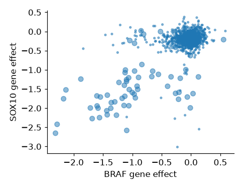
ASOX10 dependency score

BCancer lineage — Skin, Lung, Bowel…

CCell doubling time, in hours

DGene expression, in TPM

/poll

Question 2 — the hidden message

The message this figure should show: skin cancer lines need both BRAF and SOX10. Can you see it?

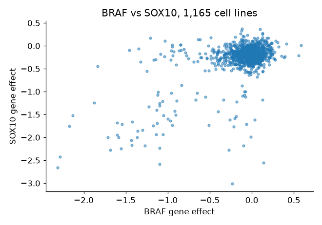
Scatter of BRAF against SOX10 gene effect, all cell lines in one colour

Every cell line is the same colour, so you can't tell which dots are skin cancer. What would you change?

Question 2 — the hidden message

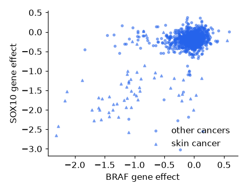
Four ways to fix it. Which gives the clearest message?

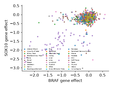
AEvery cancer type its own colour

BSkin cancer in colour, the rest grey

CSkin cancer as bigger dots

DSkin cancer as triangles

/poll

Question 3 — the wrong kind of plot

The message this figure should show: skin cancer lines need SOX10 more than other cancers. Can you see it?

Line plot of mean SOX10 gene effect across 30 cancer types in alphabetical order

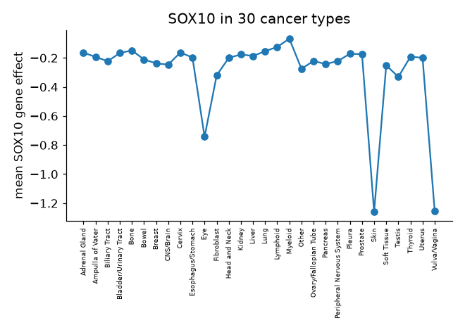
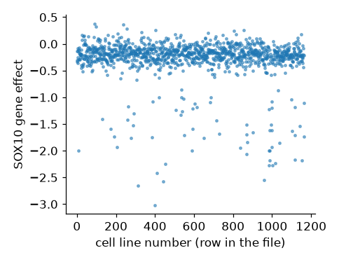
The line joins one cancer type to the next. Does "from Prostate to Skin" mean anything? What kind of data is on the x-axis?

Question 3 — the wrong kind of plot

Four ways to fix it. Which gives the clearest message?

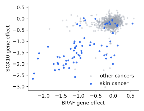
AA histogram of all SOX10 values

BOne bar per cancer type, alphabetical

CSkin vs all other cancers, box with dots

DSOX10 against the row number

/poll

Part 2

Building a basic figure

The code behind every figure: make it, put data on it, label it. By the end you will have drawn the first clue in the SOX10 case.

matplotlib has three receptions

Like the hotel in Lecture 5, you only talk to a reception. Every line of plotting code goes to one of three.

Handing a shirt across a hotel front desk

ax.one panel: draw and label it. Your main reception.

ax.scatter() ax.hist() ax.boxplot() ax.set_xlabel() ax.set_title() ax.legend()

fig.the whole figure, all its panels at once.

fig.set_size_inches() fig.suptitle() fig.tight_layout()

plt.the extras: make it, save it, show it.

plt.subplots() plt.savefig("fig.png") plt.show()

⏳Python editor will load when you reach this slide.

Build your first plot

Three steps, three runs: run it, remove the # in front of step 2, run again, then step 3.

1 · An empty figure

plt.subplots() hands you the figure and one empty panel.

2 · Put the data on it

ax.plot(hours, cells): two lists of the same length, x first, then y.

3 · Label it

Each label is an ax.set_…() on the same panel. No labels, no result.

⏳Python editor will load when you reach this slide.

Every other plot type works the same way: swap ax.plot for ax.scatter, ax.hist or ax.boxplot; steps 1 and 3 stay the same. Looking for something an ax can do? Look here first: matplotlib.org/stable/api/axes_api.html

Your first real figure: the SOX10 histogram

The same three steps, now on a DataFrame column. A histogram cuts the range of values into bins and counts how many cell lines fall into each: one bar per bin.

⏳Python editor will load when you reach this slide.

🔍 Clue 1. Most cell lines sit near 0: switching SOX10 off does nothing to them. But a long tail runs out to −3: about 90 cell lines die without it. Who are they?

Too few bins hide the tail; too many turn it into noise. There is no right number, only one that shows the shape.

Every part of a figure has a method

The histogram you just made, taken apart. Each part belongs to the panel, so each is an ax.set_…() call; only the whole sheet is fig.

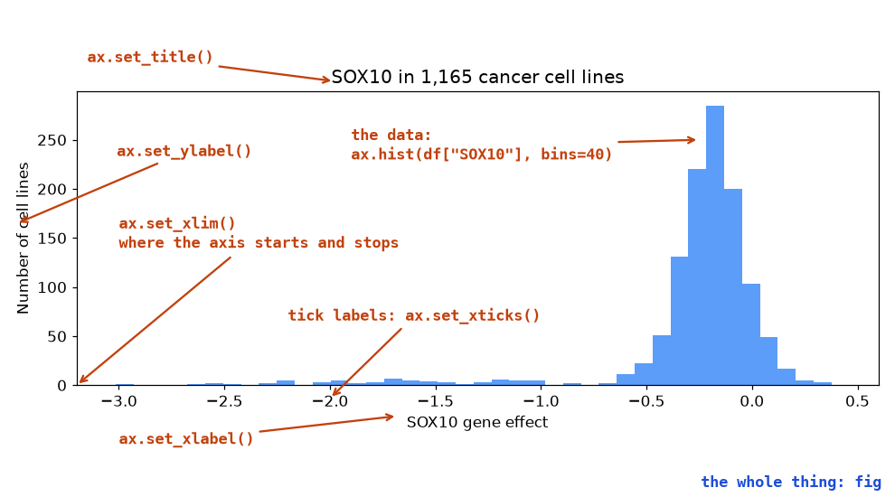
The SOX10 histogram with each part labelled by the method that sets it: set_title, set_xlabel, set_ylabel, set_xlim, set_xticks, hist

Can't remember the name? Type ax.set_ and let VS Code or Colab suggest the rest, or look it up in the Axes API.

The ax plot methods you will use most

Choose by the data you hold. The other two steps never change: make the figure, then label it.

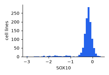
how SOX10 is spread across all cell lines

ax.hist(values, bins=40)

one continuous column

how SOX10 is spread across all cell lines

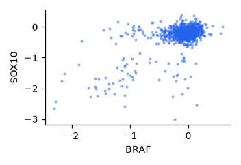
BRAF against SOX10, one dot per cell line

ax.scatter(x, y)

two continuous columns

BRAF against SOX10, one dot per cell line

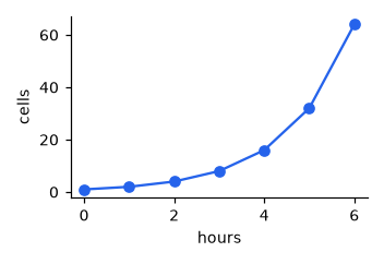
ax.plot(x, y)

a column in order, like time

a culture growing hour by hour

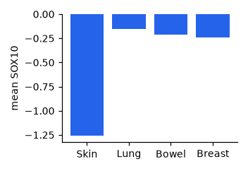
ax.bar(names, heights)

one number per category

mean SOX10 in four cancer types

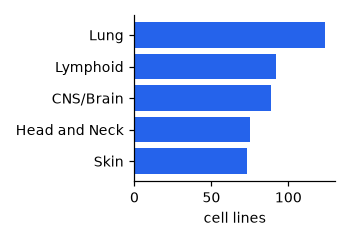
ax.barh(names, widths)

the same, with long names

cell lines per cancer type

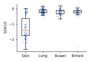
SOX10 in four cancer types, every line a dot

ax.boxplot(groups)

a continuous column, split by category

SOX10 in four cancer types, every line a dot

Many more on the same page: matplotlib.org/stable/api/axes_api.html

Quiz 2

Building a basic figure, three questions

Make it, put data on it, label it.

import matplotlib.pyplot as plt

fig, ax = plt.subplots()
ax.hist(df["SOX10"], bins=40)
ax.set_xlabel("SOX10 gene effect")

/poll

Question 1 — fig and ax

What does plt.subplots() hand you?

Afig is the data, ax is the axis labels

Bfig is the whole figure, ax is one panel you draw on

Ctwo separate figures

Da finished plot, ready to show

/poll

Question 2 — Who owns the title?

Give the panel a title.

Aplt.set_title("Growth")

Bfig.set_title("Growth")

Cax.set_title("Growth")

Dax.title("Growth")

/poll

Question 3 — More detail

The histogram hides the tail.

Afig.set_size_inches(12, 6)

Bax.set_xlim(-3, 0.5)

Cax.hist(df["SOX10"], bins=80)

Dax.set_title("SOX10, in detail")

/poll

Part 3

Extending a basic figure

One figure rarely tells the whole story. Mark a group, add colour and a legend, split by category, put two panels side by side, and the SOX10 suspects step out of the crowd.

Two columns — ax.scatter()

One column is a distribution. Two columns ask a different question: do they move together? One dot per cell line, x against y.

⏳Python editor will load when you reach this slide.

s=6 shrinks the dots and alpha=0.4 makes them see-through — with 1,165 points an opaque blob tells you nothing. Then remove the #s: a second ax.scatter on the same panel draws the skin lines on top, with bigger dots (s=30) in the next colour. 🔍 Clue 2: the cloud in the bottom left is skin cancer, lines that need SOX10 and BRAF.

Colour — a third column

The same scatter as before, drawn twice: once for everything else, once for skin on top. Two calls to the same ax, and lineage becomes visible without a third axis.

⏳Python editor will load when you reach this slide.

label= goes on the scatter call, and ax.legend() draws whatever has already been labelled. Forget the label and the legend comes up empty — remember that for the quiz.

A mean hides the spread

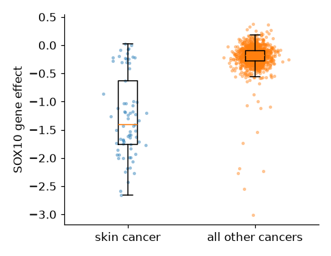
A histogram shows every cell line together. A boxplot splits them into groups and draws each group's spread: the box is the middle half, the line the median, the whiskers the rest.

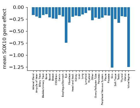
⏳Python editor will load when you reach this slide.

The skin box sits far below the others. But it is also tall: skin is not uniformly dependent, and a mean of −1.26 would hide that.

A mean hides the cell lines: show every one

A box plot with every cell line drawn on top as a dot. The dots are nudged sideways at random so they don't sit on top of each other.

⏳Python editor will load when you reach this slide.

🔍 Clue 3: most skin lines need SOX10 badly, but 18 of 73 hardly need it, and 8 of those are not melanoma at all. A box with dots on top is also exactly the plot your final project asks for.

Two panels — plt.subplots(1, 2)

Ask for two and you get an array of axes back: axes[0] is the left panel, axes[1] the right. Two methods you already know, on two panels.

⏳Python editor will load when you reach this slide.

The long left tail on the histogram is the skin box on the right — neither panel says that alone.

Finishing touches: the whole figure

The panels are done; now the fig reception. A title that states the finding, a size that fits the page, spacing that stops labels overlapping, and a file you can put in a report.

⏳Python editor will load when you reach this slide.

dpi=300 is dots per inch: high enough for print. A title that says the result ("Skin cancer lines need SOX10") beats one that names the variables ("SOX10 by lineage").

Quiz 3

Extending a figure, three questions

Groups, legends, panels: the moves that found the SOX10 suspects.

fig, ax = plt.subplots()
ax.scatter(rest["BRAF"], rest["SOX10"], color="grey", label="other")
ax.scatter(skin["BRAF"], skin["SOX10"], color="blue", label="skin")
ax.legend()

/poll

Question 1 — Add to the same panel

One panel, a second group of cell lines.

fig, ax = plt.subplots()
ax.scatter(skin["BRAF"], skin["SOX10"], label="skin")
# add the lung lines here

fig, ax = plt.subplots()
ax.scatter(lung["BRAF"], lung["SOX10"])

Bax.scatter(lung["BRAF"], lung["SOX10"], label="lung")

Cfig.scatter(lung["BRAF"], lung["SOX10"], label="lung")

Dax.scatter(lung["BRAF"], lung["SOX10"], overwrite=False)

/poll

Question 2 — A grid of panels

Count them, then find the last one.

A7 panels; axes[3][4]

B12 panels; axes[2][3]

C12 panels; axes[3][4]

D12 panels; axes[4][3]

/poll

Question 3 — Why only skin?

Read the biology off the figure.

ASOX10 is mutated in melanoma but not in other cancers

BSOX10 runs the melanocyte identity programme, and melanoma keeps that programme

COnly skin cells carry the SOX10 gene

DSkin lines grow fastest, so any knockout hurts them more

/poll

Case closed: melanoma needs SOX10

62 of the 74 melanoma lines need SOX10, whether the melanoma grew in the skin, the eye or elsewhere. Of the other 1,091 cell lines, only 31 do.

🔍 Clue 1A long tail: about 90 of 1,165 cell lines die without SOX10.

🔍 Clue 2In the scatter, the tail is skin cancer, and those lines need BRAF too.

🔍 Clue 3Split by lineage: skin needs it most. The skin lines that don’t are mostly not melanoma at all.

Why? SOX10 is the switch that makes a pigment cell (a melanocyte) a pigment cell. Melanoma is a cancer of melanocytes, and it still depends on the switch that made it. Each clue was one figure.

Your final project: does your gene respond to p53 loss?

Everything from today comes back: pandas to pick out the groups, a box plot with the points on top to show them, and next week's statistics to say whether the difference is real.

The question

Does your gene respond to loss of p53 in your cancer type, and if so, does it go up or down? Each of you gets your own gene and cancer type.

one sentence answer

The data

Real tumours from TCGA: gene expression in tumours with and without TP53 mutations, and in normal tissue. Two files: a messy patient table and a tidy expression table.

TCGA

The work

Five functions in a notebook: clean the patient table, describe your gene across cancers, compare two groups, draw the comparison, and put it all together.

Colab or VS Code

The marks

A complete, well-written and well-explained core is worth about 70. One optional extension takes you higher. The tasks are independent: if one gets stuck, move on to the next.

70 % of the module

The brief, your data files, the dates and the submission are all on Canvas.

What you can do now

categorical or continuous?decide what you hold, then choose the plot and the aesthetic

fig, ax = plt.subplots()every figure starts here; the axes do the drawing

ax.hist · ax.scatter · ax.barh · ax.boxplotpick the plot from the kind of columns you have

ax.scatter(..., label=) + ax.legend()mark a group and say what it is

plt.subplots(1, 2) and axes[0], axes[1]two panels, side by side

fig.suptitle() · plt.savefig()finish the figure and save it

One gene, one question, five figures: that is how you will work in your project too. Next week: is a difference real, or could it be chance? Statistics.